Excel Expert page contents

XLXpart

Microsoft Excel is one of the Best application provided within Msoffice suite. Excel is very popular software among Corporate Sector. We have gained some really fantastic experience. Believe us it is very wonderful application and you will really enjoy using it. This blog is trying to convey some of its Excel's Dynamic Functions, Versatile Functionality, Flexibilities and some fun tricks. We shall also try to resolve your queries.

Search Here

Loading

6/14/13

Use "Calculation on Top Row" for Ease of work.


There are 2 most important use of any Spreadsheet first store the important Data and Another one Calculation using several methods available with Excel. Most commonly used method is use of formulas.

A commonly used design of spreadsheet is consists of Heading Row that contains Column Titles, Data and at the bottom of it Calculation resulted by some formulas. This is an old practice of the time when all the works were done manually, thus it became necessary to calculate totals when all work is done. With computers we use same sheet repeatedly and make corrections and calculate. I learnt with my experience that keeping calculation on above titles or just below gives an easy view of results and also give flexibility to work.

1. Scope of Calculation done at the bottom of Data has a limited scope. Every time if we add new rows of data at the bottom, we need to edit each formula to take the new row in calculation. It is convenient for few numbers of formulas but what if have to change more formulas, it becomes a cumbersome job.
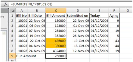
whereas while entering formulas on top of data we can take All the data rows in calculation and never need to update a formula.

2. We need to scroll the entire sheet down to view results. However, Smartly we freeze Title Panes and set both Title and Calculation in vision. but still it is not easy.
We need to only freeze top or/and left pans and continue our work at the rest of the data at any part of worksheet and both calculation and titles will remain in our vision.

3. While printing if we want to have both Titles and Calculation, we need to print the entire sheet. but if totals are on top; we just to take a printout of top rows.

However taking total on top looks awkward but it is only because we don't see the data in that way. Also we shall have to control on the habit of doing rough work on the same sheet below data otherwise rough  figure can be taken in calculations.

2/17/11

Change Local Comma, Currency and Date Settings Effective for Excel.

In our world there are many countries and have different formats for Date and Currency.
Like Britishers have dd/MM/yyyy date format and Americans prefer MM/dd/yyyy format whereas ISO recommends yyyy/mm/dd format. But since Microsoft is America based, All computer are default set to MM/dd/yyyy date format.

Same with Currency format. Every country has it's own Currency Recognition Symbol and Comma/Decimal Separators.
Like in India ones,tens, hundred (3) are grouped in first comma place and  Thousand and Bigger amounts are grouped in 2 comma places (1,23,45,67,890.00) but in American and some other patters all the numbers are grouped in 3 (1,234,567,890)

In Europe Commas are used to separate to decimals, and decimal is used as comma.

It is enough that laid Microsoft to provide flexibility in his operating systems to change the number and date systems as per Regional location.

How can one change these settings....?

Open Control Panel - Double Click on Regional and Language Options

It is recommended that AT Regional Options Tab Firstly select the Location (your country name)

Click on Customize

1. in Numbers tab you can Set Decimal Symbol (generally "."), Digit Grouping Symbol (generally ","), Digit Grouping (Select 3,3 or 2,3 Pattern), and other options
2. in Currency Tab you can Provide the Currency Symbol and Digit Grouping and other Options.
3. in Date tab - Short Date format Specify your desired date format. (it is very important to enter the pattern correctly, because Excel and other applications that refer Windows Date Format shall recognize and convert the date in format Specified by you in Short Date format)

Save the settings now Run Excel and Check the Settings. How effectively it works and how flexible it is.

10/7/10

Retrieving Values other Files using Address & Indirect Functions.

Retrieving Values other Files using Address & Indirect Functions.

First of all you must understand the Address and Indirect Functions

Address Function: ADDRESS function is used to obtain the address of a cell in a worksheet, given specified row and column numbers. For example, ADDRESS(1,1) returns $A$1 and ADDRESS(10,2) returns $B$10.

Syntax: =ADDRESS(row_num, column_num, [abs_num], [a1], [sheet_text])

row_num: Required. A numeric value that specifies the row number to use in the cell reference.
column_num: Required. A numeric value that specifies the column number to use in the cell reference.
abs_num: Optional. A numeric value that specifies the type of reference to return.
1 or omitted Absolute (the exact address of a cell, regardless of the position of the cell that contains the formula. Example $A$1.)
2 Absolute row & relative column (A$1)
3 Relative row; absolute column ($A1)
4 Relative (A1)
Sheet_Text: Optional Name of the Sheet that is required in Cell Address


Indirect Function: Retrieves the Value of Any range/Cell Specified by the Text String.

Syntax: INDIRECT(ref_text, [a1])

ref_text: Text String that is written a Address of any Cell or range, Like "A1", "$A$1", "Sheet1!$a$1"
a1: Optional logical value that specifies what type of reference is contained in the cell ref_text.
a1 = FALSE: ref_text is as an R1C1-style reference.
a1 = TRUE: ref_text is as an A1-style reference.


Let’s come back to our Objective.

To this purpose we need to have 2 more Parameters that are File Path & File Name

Generally in any Formula we Refer to any cell in

c:\Folder Name\[File Name.ext]SheetName!RowColumn

So Our Formula will be

=Indirect(“File_Path” &”\” & “File Name.ext” & Address(Row,Column,1,1,”Sheet1)

For Example we we want to Retrive some value from any Excel File that is stored on C:

=Indirect(“C:\My File.xlsx”,address(1,1,1,1,”Sheet1”))

This will retrieve the value from Cell A1 of C:\My File.xlsx

1/1/10

IF Function in Excel

=IF(logical test, value if true, [value if false])


The IF function returns one value if a condition you specify evaluates to TRUE, and another value if that condition evaluates to FALSE. For example, the formula =IF(A1>10,"Over 10","10 or less") returns "Over 10" if A1 is greater than 10, and "10 or less" if A1 is less than or equal to 10.


The IF function syntax has the following arguments (argument: A value that provides information to an action, an event, a method, a property, a function, or a procedure.):


» logical_test Required. Any value or expression that can be evaluated to TRUE or FALSE. For example, A10=100 is a logical expression; if the value in cell A10 is equal to 100, the expression evaluates to TRUE. Otherwise, the expression evaluates to FALSE. This argument can use any comparison calculation operator.


» value_if_true Required. The value that you want to be returned if the logical_test argument evaluates to TRUE. For example, if the value of this argument is the text string "Within budget" and the logical_test argument evaluates to TRUE, the IF function returns the text "Within budget." If logical_test evaluates to TRUE and the value_if_true argument is omitted (that is, there is only a comma following the logical_test argument), the IF function returns 0 (zero). To display the word TRUE, use the logical value TRUE for the value_if_true argument.


» value_if_false Optional. The value that you want to be returned if the logical_test argument evaluates to FALSE. For example, if the value of this argument is the text string "Over budget" and the logical_test argument evaluates to FALSE, the IF function returns the text "Over budget." If logical_test evaluates to FALSE and the value_if_false argument is omitted, (that is, there is no comma following the value_if_true argument), the IF function returns the logical value FALSE. If logical_test evaluates to FALSE and the value of the value_if_false argument is omitted (that is, in the IF function, there is no comma following the value_if_true argument), the IF function returns the value 0 (zero).

12/30/09

Limits in Excel.

Worksheet and workbook specifications
  •  Open workbooks Limited by available memory and system resources
  • Worksheet size 65,536 rows by 256 columns
  • Column width 255 characters
  • Row height 409 points
  • Page breaks 1000 horizontal and vertical
  • Length of cell contents (text) 32,767 characters. Only 1,024 display in a cell; all 32,767 display in the formula bar.
  • Sheets in a workbook Limited by available memory (default is 3 sheets)
  • Colors in a workbook 56
  • Cell styles in a workbook 4,000
  • Named views (view: A set of display and print settings that you can name and apply to a workbook. You can create more than one view of the same workbook without saving separate copies of the workbook.) in a workbook Limited by available memory
  • Custom number formats Between 200 and 250, depending on the language version of Excel you have installed.
  • Names in a workbook Limited by available memory
  • Windows in a workbook Limited by system resources
  • Panes in a window 4
  • Linked sheets Limited by available memory
  • Scenarios (scenario: A named set of input values that you can substitute in a worksheet model.) Limited by available memory; a summary report shows only the first 251 scenarios
  • Changing cells in a scenario 32
  • Adjustable cells in Solver 200
  • Custom functions Limited by available memory
  • Zoom range 10 percent to 400 percent
  • Reports Limited by available memory
  • Sort references 3 in a single sort; unlimited when using sequential sorts
  • Undo levels 16
  • Fields in a data form 32
  • Custom toolbars in a workbook Limited by available memory
  • Custom toolbar buttons Limited by available memory
Calculation specifications
  • Number precision 15 digits
  • Largest number allowed to be typed into a cell 9.99999999999999E+307
  • Largest allowed positive number 1.79769313486231E+308
  • Smallest allowed negative number -2.2251E-308
  • Smallest allowed positive number 2.229E-308
  • Largest allowed negative number -1E-307
  • Length of formula contents 1,024 characters
  • Iterations 32,767
  • Worksheet arrays Limited by available memory. Also, arrays cannot refer to entire columns. For example, an array cannot refer to the entire column C:C or to the range C1:C65536. However, an array can refer to the range C1:D65535 because the range is one row short of the maximum worksheet size and does not include the entire C or D column.
  • Selected ranges 2,048
  • Arguments in a function 30
  • Nested levels of functions 7
  • Number of available worksheet functions 329
  • Earliest date allowed for calculation January 1, 1900 (January 1, 1904, if 1904 date system is used)
  • Latest date allowed for calculation December 31, 9999
  • Largest amount of time that can be entered 9999
Charts linked to a worksheet Limited by available memory
  • Worksheets referred to by a chart 255
  • Data series (data series: Related data points that are plotted in a chart. Each data series in a chart has a unique color or pattern and is represented in the chart legend. You can plot one or more data series in a chart. Pie charts have only one data series.) in one chart 255
  • Data points (data points: Individual values that are plotted in a chart. Related data points make up a data series. Data points are represented by bars, columns, lines, slices, dots, and other shapes. These shapes are called data markers.) in a data series for 2-D charts 32,000  
  • Data points in a data series for 3-D charts 4,000  
  • Data points for all data series in one chart 256,000 
  • Line styles 8  
  • Line weights 4 
  • Area patterns (screen display) 18  
  • Total area pattern and color combinations (color display) 56,448 
  • Pattern and color combinations (color printer) 56,448 (the actual number depends on your printer and its software)  
  • Page fields (page field: A field that's assigned to a page orientation in a PivotTable or PivotChart report. You can either display a summary of all items in a page field, or display one item at a time, which filters out the data for all other items.) in a PivotChart report (PivotChart report: A chart that provides interactive analysis of data, like a PivotTable report. You can change views of data, see different levels of detail, or reorganize the chart layout by dragging fields and by showing or hiding items in fields.) 256 (may be limited by available memory)  
  • Data fields (data field: A field from a source list, table, or database that contains data that is summarized in a PivotTable report or PivotChart report. A data field usually contains numeric data, such as statistics or sales amounts.) in a PivotChart report 256  
  • Calculated item formulas in a PivotChart report Limited by available

12/18/09

Date Functions

In Addition to Dynamic date handling Excel provides a wide range of Date related functions to enable us to manipulate dates as most extend.

  • Date Function: This function used to compose date
Syntex: Date(year,month,day)
Example:
=date(2009,12,17)
composes: 17th December'2009

  • you can also use DateValue function to convert String date into date

Syntex: DateValue("date")
Example:
=DateValue("2009/12/17")
Retunrs: 40164  (that is equals to 17th December'2009)

this value can be used further in any function as parameter.

Best part of this function is it flexibility that allows to enter the date in any format, As we take above example we could enter date "17/12/2009", "17 dec 09", "17-December-2009"


  • Day:  This function returns the day from any date provided
Syntex: Day(date) or Day("mm/dd/yyyy")
Example: Day("12/01/2009")
Returns: 01

Note: Excel uses the System's date format by default it is 'M/d/yyyy' you can change this format using control panel - Regional Settings - Dates


Month: Like day function month returns the month from any date provided
Syntex: Month(date) or Month("mm/dd/yyyy")
Example: Month("12/01/2009")
Returns: 12

Year: Like day & Month functions year returns the year from any date provided

Syntex: Year(date) or Year("mm/dd/yyyy")
Example: Year("12/01/2009")
Returns: 2009

Weekday: Weekday function returns the Weekday that is falling on the date provided

Syntex: =Weekday(date)
Example: =Weekday("2009/12/17")
Returns 5 i.e. Thursday
begning from Sunday = 1, Monday = 2 and so on Saturday = 7

Today(): This  function returns the current date. And as the date is changed Excel automatically updates today function on next calculation to the prevailling date this way it will always returen the present date.

Value returned by this function is variable it changes as the date changes to insert constant current date  that doesn't change with change date use Keyboard Shortcut Ctrl + ;

Date.Diff(): this function calculates the differances in months & year between two dates.
Syntex: date.diff(date1,date2)
Example: =DATE.DIFF("10/10/2008",today())
Return: 1 year 2 months  (Assuming today is 17-December-2009)
This function does not calculates differances in days.

For Additional Details about Dates Visit: http://xlxpart.blogspot.com/2009/12/dates-in-excel.html

12/8/09

Dates in Excel

Handling Date methods in Excel is one of the very interesting matters. The Best part of it is you can perform calculation on it.

As Default Excel stores the dates in simple numbers and it is then displayed in Systems date format.

Default system’s format is MM/dd/yyyy but in excel you can change this format as per your convenience.

Likewise Enter any date in any cell

Right click – Format Cells

From Numbers Tab Click on Date and from given several options select any format of date as previewed.

Press OK then Cell’s format of date will be changed

Or you can define your own format. For doing this.

Instead of selecting date from Numbers tab Select Cutom

And enter

“dd/MM/yyyy” or “dd-MM-yyyy” (without Quotes) and see the cell format exactly same.

Now for understanding how to deal with format see the followings:

Date is comprises of three parts (Days, Months and Year) and additional to it a separator is used (by default these separators are “/” and “-“).

d: Represents Day in date
d: day will be displayed in single digit and if day is greater then 9 then only it will be display in tow digits (Like: 2,12)
dd: day will be displayed in two digits and if day is less then 9 then a leading Zero will be added (Like: 02,12)
ddd: days will be showed in weekday format (sun, mon, tue)
dddd: days will be showed in Complete weekday Name format (sunday, monday, tuesday)

m: Denotes Month
m: Month will be displayed in single digit and if Month is greater then 9 then only it will be display in tow digits (Like: 2,12)
mm: Month will be displayed in two digits and if Month is less then 9 then a leading Zero will be added (Like: 02,12)
mmm: Month will be showed in Short Month Name format (Jan, Feb, Mar)
mmmm: Month will be showed in Complete Month Name format (January, February, March)

and y finally denotes year
y: Year will be displayed in single digit and if Year is greater then 9 then only it will be display in tow digits (Like: 2,12)
yy: year will be displayed in two digits and if year is less then 9 then a leading Zero will be added (Like: 02,12)
yyy: Year will be showed in year with century format Like 2009, 2012, 1999

Normally System’s setting allows the default century format like if you type 11/11/25 then date will be 11/11/2025 and if you type 11/11/99 the date will be 11/11/1999, That is because of regional settings. Whenever any two digit year is entered system interprets it based on the system’s setting

To change the Date format and Two Digit year behavior you can go to Control Panel – Regional and Language Option – and Select date.

Change the behavior as per your requirements, But still be careful because if system’s default date format is changed then may some software not work or may behave unscientifically.

Calculation on Dates

As I already stated that calculation on any date is possible

For example Cell A1 has stored date 8th December – 2009 then

Use following formulas

=A1 + 1: 9th December - 2009

=A1 - 1: 7th December - 2009

Suppose you have some date in A2 (15/12/2009)

=A2 –A1 = 07/01/1900 Change it to Number format and you can find the differences of two dates i.e. 7.

You can divide, multiply, add or subtracts date from one another and after changing the cell format to numbers you can get the results.

You can also sue Date.Diff formula to obtain deference of date.

For Additional Details about Excel Date related function Visit:
http://xlxpart.blogspot.com/2009/12/date-functions.html

12/4/09

Is it possible to create a pivot table using source data from more than one worksheet?

Yes you can create pivot using multiple Worksheets. But this function is not as flexible as you create pivot table using single sheet.
Sturcture of all the tables must remain same to take the advantage of this feature.
use keyboard short keys to aproach if you are using 2007 version otherwise the multiple table merging option may not be visile to you.

Press Alt + D followed by P
Select third option "Multiple Consoliation Ranges"
Click Next
Select "Select a Single Page Field for me"
Click Next

Now Select First range and Click on ADD
Add
and Select & Add as many ranges you want to consolidate.
Click Next/Finish

Now a Pivot is created using default fields.
Remeber Only First column values will be treated as row label
and First Column Values will be treated as Columns.

you can drag Column values before and after only column values and can change the way of calculation for the column labels.

As I have already stated you that this is not much flexible function but still very useful. you can experience it yourself while using it.

12/2/09

Excel Sumif

At several times we require calculating the total of our data tables based on some criteria.


Lets take an example:

Suppose we have a excel sheet that has the data of bills submitted by us and we calculating the aging of our bills from the date of submission. Only the bill submission date is older than 30 days then we forward the total start follow up by commercial department.


Here in above sheet we have the Bill submission date we subtract the submission date from today’s date in column E (Instead of entering today’s date in saperate column we can also subtract it directly from Today() function.

We put the Function

=Sumif(F2:F8,”>30”,C2:C8)

This function has three parts

=SUMIF(range,criteria,sum_range)


1. Range: first specify the range that we have to check if it matches to Criteria

2. Criteria: in this we provide the logical equation for the range we want to check

“=30” : Equals to 30

“>=30” : Grater then or equals to 30

“<=30” : Less then or equals to 30

“<30” : Less then 30

“<>30” : Not Equals to 30

>,< and = are the logical operator that can compare two values and can gives True or False results.

3. Sum_Range: in this part we specify range of which we have to take total.

If we ommit the last optional argument (sum_range) the SUMIF would sum all cells in the range F1:F8 which are greater than 30.

11/29/09

Insert the Name of WorkBook in the Cell.

This is very rarely required value in excel but Essencial. this can be used in the formulas to refer the exact location of any file.
Excel doesn't provide direct inbuild feature to retrive the filename in any cell. But it provids us a simple way to retrive it through comination of formulas.

Use the following formula:

=SUBSTITUTE(LEFT(CELL("FileName"),FIND("]",CELL("filename"))-1),"[","")

Here we have used four function to achive our goal

1. sustitute: this function simply finds a part of text in the complete sentencd and replaces with another
like
=sustitute("ABCD","A","X")

In above example from "ABCD" the "A" will be replaced by "X", and the return value of the formula will be XBCD

2. Left: This simply return the leftmost Nth numbers from any text
Like
=Left("ABCD",2) *here we instructed excel to retrive only 2 left characters from ABCD
Thus formula will return - AB

3. Find: this function will simply give the Nth position of the searched text from sentance
=Find("B","ABCD") this function will return the position of B from the left so the value will be 2, as B is on 2nd position from left.

4. Cell: This function retrives the information from Excel Application and return it to us.
there are several perameters provided to for different purposes. in our case we used it to retrive the Name of file.

=Cell("FileName")
this will return the Location + Name of File (Enclosed within Square Brackets) + SheetName
like
C:\Amit\Office\[BlogData.xls]sheet1

useing the find function we retrived the position of ]
from the Left to till the position ] we retrived the text using left function
and using substitute function we replaced [ as "" (2 double quotes continously denot the blank) from the returned value.

we can use this formula in any cell and we can have the name of file in the cell we enter the foumula
C:\Amit\Office\BlogData.xls