Handling Date methods in Excel is one of the very interesting matters. The Best part of it is you can perform calculation on it.
As Default Excel stores the dates in simple numbers and it is then displayed in Systems date format.
Default system’s format is MM/dd/yyyy but in excel you can change this format as per your convenience.
Likewise Enter any date in any cell
Right click – Format Cells
From Numbers Tab Click on Date and from given several options select any format of date as previewed.
Press OK then Cell’s format of date will be changed
Or you can define your own format. For doing this.
Instead of selecting date from Numbers tab Select Cutom
And enter
“dd/MM/yyyy” or “dd-MM-yyyy” (without Quotes) and see the cell format exactly same.
Now for understanding how to deal with format see the followings:
Date is comprises of three parts (Days, Months and Year) and additional to it a separator is used (by default these separators are “/” and “-“).
d: Represents Day in date
d: day will be displayed in single digit and if day is greater then 9 then only it will be display in tow digits (Like: 2,12)
dd: day will be displayed in two digits and if day is less then 9 then a leading Zero will be added (Like: 02,12)
ddd: days will be showed in weekday format (sun, mon, tue)
dddd: days will be showed in Complete weekday Name format (sunday, monday, tuesday)
m: Denotes Month
m: Month will be displayed in single digit and if Month is greater then 9 then only it will be display in tow digits (Like: 2,12)
mm: Month will be displayed in two digits and if Month is less then 9 then a leading Zero will be added (Like: 02,12)
mmm: Month will be showed in Short Month Name format (Jan, Feb, Mar)
mmmm: Month will be showed in Complete Month Name format (January, February, March)
and y finally denotes year
y: Year will be displayed in single digit and if Year is greater then 9 then only it will be display in tow digits (Like: 2,12)
yy: year will be displayed in two digits and if year is less then 9 then a leading Zero will be added (Like: 02,12)
yyy: Year will be showed in year with century format Like 2009, 2012, 1999
Normally System’s setting allows the default century format like if you type 11/11/25 then date will be 11/11/2025 and if you type 11/11/99 the date will be 11/11/1999, That is because of regional settings. Whenever any two digit year is entered system interprets it based on the system’s setting
To change the Date format and Two Digit year behavior you can go to Control Panel – Regional and Language Option – and Select date.
Change the behavior as per your requirements, But still be careful because if system’s default date format is changed then may some software not work or may behave unscientifically.
Calculation on Dates
As I already stated that calculation on any date is possible
For example Cell A1 has stored date 8th December – 2009 then
Use following formulas
=A1 + 1: 9th December - 2009
=A1 - 1: 7th December - 2009
Suppose you have some date in A2 (15/12/2009)
=A2 –A1 = 07/01/1900 Change it to Number format and you can find the differences of two dates i.e. 7.
You can divide, multiply, add or subtracts date from one another and after changing the cell format to numbers you can get the results.
You can also sue Date.Diff formula to obtain deference of date.
For Additional Details about Excel Date related function Visit:
http://xlxpart.blogspot.com/2009/12/date-functions.html

12/8/09
12/4/09
Is it possible to create a pivot table using source data from more than one worksheet?
Yes you can create pivot using multiple Worksheets. But this function is not as flexible as you create pivot table using single sheet.
Sturcture of all the tables must remain same to take the advantage of this feature.
use keyboard short keys to aproach if you are using 2007 version otherwise the multiple table merging option may not be visile to you.
Press Alt + D followed by P
Select third option "Multiple Consoliation Ranges"
Click Next
Select "Select a Single Page Field for me"
Click Next
Now Select First range and Click on ADD
Add
and Select & Add as many ranges you want to consolidate.
Click Next/Finish
Now a Pivot is created using default fields.
Remeber Only First column values will be treated as row label
and First Column Values will be treated as Columns.
you can drag Column values before and after only column values and can change the way of calculation for the column labels.
As I have already stated you that this is not much flexible function but still very useful. you can experience it yourself while using it.
12/2/09
Excel Sumif
At several times we require calculating the total of our data tables based on some criteria.
Lets take an example:
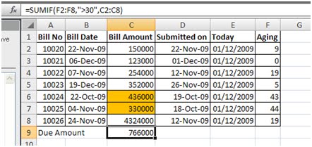
Suppose we have a excel sheet that has the data of bills submitted by us and we calculating the aging of our bills from the date of submission. Only the bill submission date is older than 30 days then we forward the total start follow up by commercial department.

Here in above sheet we have the Bill submission date we subtract the submission date from today’s date in column E (Instead of entering today’s date in saperate column we can also subtract it directly from Today() function.
We put the Function
=Sumif(F2:F8,”>30”,C2:C8)
This function has three parts
=SUMIF(range,criteria,sum_range)
1. Range: first specify the range that we have to check if it matches to Criteria
2. Criteria: in this we provide the logical equation for the range we want to check
“=30” : Equals to 30
“>=30” : Grater then or equals to 30
“<=30” : Less then or equals to 30
“<30” : Less then 30
“<>30” : Not Equals to 30
>,< and = are the logical operator that can compare two values and can gives True or False results.
3. Sum_Range: in this part we specify range of which we have to take total.
If we ommit the last optional argument (sum_range) the SUMIF would sum all cells in the range F1:F8 which are greater than 30.
Lets take an example:
Suppose we have a excel sheet that has the data of bills submitted by us and we calculating the aging of our bills from the date of submission. Only the bill submission date is older than 30 days then we forward the total start follow up by commercial department.
Here in above sheet we have the Bill submission date we subtract the submission date from today’s date in column E (Instead of entering today’s date in saperate column we can also subtract it directly from Today() function.
We put the Function
=Sumif(F2:F8,”>30”,C2:C8)
This function has three parts
=SUMIF(range,criteria,sum_range)
1. Range: first specify the range that we have to check if it matches to Criteria
2. Criteria: in this we provide the logical equation for the range we want to check
“=30” : Equals to 30
“>=30” : Grater then or equals to 30
“<=30” : Less then or equals to 30
“<30” : Less then 30
“<>30” : Not Equals to 30
>,< and = are the logical operator that can compare two values and can gives True or False results.
3. Sum_Range: in this part we specify range of which we have to take total.
If we ommit the last optional argument (sum_range) the SUMIF would sum all cells in the range F1:F8 which are greater than 30.
11/29/09
Insert the Name of WorkBook in the Cell.
This is very rarely required value in excel but Essencial. this can be used in the formulas to refer the exact location of any file.
Excel doesn't provide direct inbuild feature to retrive the filename in any cell. But it provids us a simple way to retrive it through comination of formulas.
Use the following formula:
=SUBSTITUTE(LEFT(CELL("FileName"),FIND("]",CELL("filename"))-1),"[","")
Here we have used four function to achive our goal
1. sustitute: this function simply finds a part of text in the complete sentencd and replaces with another
like
=sustitute("ABCD","A","X")
In above example from "ABCD" the "A" will be replaced by "X", and the return value of the formula will be XBCD
2. Left: This simply return the leftmost Nth numbers from any text
Like
=Left("ABCD",2) *here we instructed excel to retrive only 2 left characters from ABCD
Thus formula will return - AB
3. Find: this function will simply give the Nth position of the searched text from sentance
=Find("B","ABCD") this function will return the position of B from the left so the value will be 2, as B is on 2nd position from left.
4. Cell: This function retrives the information from Excel Application and return it to us.
there are several perameters provided to for different purposes. in our case we used it to retrive the Name of file.
=Cell("FileName")
this will return the Location + Name of File (Enclosed within Square Brackets) + SheetName
like
C:\Amit\Office\[BlogData.xls]sheet1
useing the find function we retrived the position of ]
from the Left to till the position ] we retrived the text using left function
and using substitute function we replaced [ as "" (2 double quotes continously denot the blank) from the returned value.
we can use this formula in any cell and we can have the name of file in the cell we enter the foumula
C:\Amit\Office\BlogData.xls
11/26/09
New expectetion with 2011 Version in Excel.
Hi...!
Recently newer 2010 version of Ms-excel we release. but still I m expecting some more features with the New version of Excel. I wish to have some them on excel without any additional coding requirement so that any layman can use those features.
1. Summery Wizard: There should be a tool that can summarize the multiple sheet in to one Summery Sheet for example
I have a sheet which contains Purchase Orders in a Standard Format in which some fields are defined like PO No. Date, Vendor's Name, Total Amount, Taxes, Grand Total.
Now on summery sheet I want to have the summery and total of those purchase orders and if it put a remark on summery sheet it should be updated in the respective PO. like Date of Approval Remarks, Submission Date Etc.
2. One of most exiting feature of Excel it Pivot Table but still We are limited to summarize the Single sheet with this feature. The Newer version must contain the capacity to summarize the multiple sheet with same structure in the single Pivot Table.
3. Data Validation List with some conditions like (don't Include First Row, Don't Include Blank cells in the range, or Don't Include certain criteria matched Values from the cells in the range.
Validate only with Unique Items in a Range.
4. Paste Special: There are some Options available on the Right Click - Paste Special. Options that are provided as Radio Buttons must be converted into Check Boxes so that we must be able to make multiple selection. Like if we want to Paste values and Format simultaneously we can Check Values + Formats so that we can ignore to paste column width and Formulas etc.
5. Some Additional Formulas Like
> GetSheetName to Retrieve Sheet Name.
> NumberToWords to convert Numerical Values in Words for at-least thousand crore amount.
> GetCellProperties (FillColor, FontColor, Bold, Italic, Underline, Width and Height etc.
> A formula that can define the Criteria and Ranges that can be further used in Dsum, Dcount, sumif, and countif functions. because Criteria defination in a saperate space is quite tedious and limited affair and not flexible at all.
> Three Additional Formulas or any specific Portion in Excel that can define a Variable and set its Values.
DefVariable - to Define Variable of Certain Datatype.
SetVariableValue - to change the Variable Value
GetVariableValue - to retrieve Values of certain Variable
* above must be addition to the defining Name range.
> An Additional Function Split & Retrieve Nth Part of text: A Function that can Split apart a text using a delimiter and can retrieve Nth splited value in cell.
6. Linked Cells & Ranges: Excel should avail Mutually Linked Cells: Means Two or more cells should linked in such a way that if any one of Linked cell is changed Rest all linked cells should be updated automatically.
Same should be availed with Multiple Ranges / Arrays.
7. Mini Excel / Word: A New Compact Sheet / Doc should be introduced that can run like Calculator or Notepad with Limited Options available for quick Calculations and Notes. It should not much Space nor it should take Much time to Run and open & Save the files.
Above are not for very scientific usage but are used in very routine workings, If we can have them on excel working can be done more dynamically.
11/25/09
2007 Advance Version.
As compared to Old 2003 / XP version of MS Excel in 2007 Version several New Interaction to the Features are added. In previous versions of excel Several Features were Availble but not easily visible. But in 2007 Those Feature are put in front row. Like Auto Fiter's Features that were abailable in only Custom Menu is now splited in several parts and made accessible through Simple Second Line Menu Command.
but some interesting features are added with this version.
1. In Filters we are now able to select as many items we want to select but in previous version only the person who knows Advance filter could select more then tow items.
2. Conditional Formatting is now with several designs and Styles possible. you can apply conditional formatting with more then three conditions. New Data Bars, Icon Sets and Colour Scale helps to analysis data with visual effects.
3. Sorting is now more customizable, Also possile with more then 3 sorting priorities.
4. Some newly added function like, BIN2DEC & DEC2BIN and Randbetween.
5. New Menu Style. Added a nice look to Excel. for some persons it is not convenient but it is the matter of practice only.
6. Excel Introduced a new way of Menu Item aproach but kept in considering the approach through older keyboard combination to the menu items is still possible. In some menu items the results are differant like
if you Press Alt + A + T it will show a Pivot Table Wizard but if you use the Lagacy Keyboard Combination the Classic Pivot Tale Wizard is shown.
But the great thing with this version is now Excel Sheet is more Wide and more Long
1048576 rows X 16384 columns = 17179869184 Cells to work
Still some parts in excel that are to be added in Excel but expecting Like
A formula that can convert Numerical Values in Words.
Pivot table is still requires manual refresh.
There is no formula for Getting Formatting Information of any cell or range.
Thera is no Foumula that can provide information about sheet like sheet name sheet Index no. Etc.
Anyways we are soon expecting newer Version 2010 very shortly. lets hope excel will be with us in a new Avtaar.
Some Excel Shortcut Keys
Shortcut Keys Description
F2 Edit the selected cell.
F5 Goto a specific cell. For example, C6.
F7 Spell check selected text and/or document.
F11 Create chart.
Ctrl + Shift + ; Enter the current time.
Ctrl + ; Enter the current date.
Alt + Shift + F1 Insert New Worksheet.
Shift + F3 Open the Excel formula window.
Shift + F5 Bring up search box.
Ctrl + A Select all contents of the worksheet.
Ctrl + B Bold highlighted selection.
Ctrl + I Italic highlighted selection.
Ctrl + K Insert link.
Ctrl + U Underline highlighted selection.
Ctrl + 5 Strikethrough highlighted selection.
Ctrl + P Bring up the print dialog box to begin printing.
Ctrl + Z Undo last action.
Ctrl + F9 Minimize current window.
Ctrl + F10 Maximize currently selected window.
Ctrl + F6 Switch between open workbooks / windows.
Ctrl + Page up Move between Excel work sheets in the same Excel document.
Ctrl + Page down Move between Excel work sheets in the same Excel document.
Ctrl + Tab Move between Two or more open Excel files.
Alt + = Create a formula to sum all of the above cells
Ctrl + ' Insert the value of the above cell into cell currently selected.
Ctrl + Shift + ! Format number in comma format.
Ctrl + Shift + $ Format number in currency format.
Ctrl + Shift + # Format number in date format.
Ctrl + Shift + % Format number in percentage format.
Ctrl + Shift + ^ Format number in scientific format.
Ctrl + Shift + @ Format number in time format.
Ctrl + Arrow key Move to next section of text.
Ctrl + Space Select entire column.
Shift + Space Select entire row.
Dancing Chart
Ycan make some fun with Chart using Rand or randbetween (only for 2007 or later versions) in excel.
enter the formula in A1
=rand()
or
=randbetween(1,10)
copy the cell and paste it to a1 to j10
select the same range
and press F11
A new sheet with chart is created.
now keep holding F9 key and see the changes.
now change different chart types and colors and Enjoy.
Tip: Short Keys
F11 : Creates a new Sheet with Chart for selected Range
F9 : Re-calculats the entire sheet.
Subscribe to:
Posts (Atom)